2D Problems

6.1 Review of the Basic Theory

Plane problems:

• Plane stress: A thin planar structure with constant thickness and loading within the plane of the structure (xy-plane)
  • \(\sigma_z = \tau_{zx} = \tau_{zy} = 0, \, \varepsilon_z \neq 0\)
• Plane strain: A long or thick structure with a uniform cross section and transverse loading along its length (z-direction)
  • \(\varepsilon_z = \gamma_{zx} = \gamma_{zy} = 0, \, \sigma_z \neq 0\)

Stress-Strain Relations

Plane Stress

For linear elastic homogeneous and isotropic materials:

\[ \begin{bmatrix} \varepsilon_x \\ \varepsilon_y \\ \gamma_{xy} \end{bmatrix} = \begin{bmatrix} 1/E & -\nu / E & 0 \\ -\nu / E & 1/E & 0 \\ 0 & 0 & 1/G \end{bmatrix} \begin{bmatrix} \sigma_x \\ \sigma_y \\ \tau_{xy} \end{bmatrix} \]

where

\[ G = \frac{E}{2(1 + \nu)}. \]

Only 2 independent material constants. The inverse relation:

\[ \begin{gather} \begin{bmatrix} \sigma_x \\ \sigma_y \\ \tau_{xy} \end{bmatrix} = \frac{E}{1 - \nu^2} \begin{bmatrix} 1 & \nu & 0 \\ \nu & 1 & 0 \\ 0 & 0 & (1 - \nu) / 2 \end{bmatrix} \begin{bmatrix} \varepsilon_x \\ \varepsilon_y \\ \gamma_{xy} \end{bmatrix} \\[2ex] \implies \boldsymbol{\sigma} = \mathbf{D} \boldsymbol{\varepsilon}, \quad \mathbf{D} = \frac{E}{1 - \nu^2} \begin{bmatrix} 1 & \nu & 0 \\ \nu & 1 & 0 \\ 0 & 0 & (1 - \nu) / 2 \end{bmatrix} \tag{6.1} \label{eq:plane_stress-strain} \end{gather} \]

\(\mathbf{D}\): material stiffness matrix for plane stress problems.

Plane Strain

\[ E \to \frac{E}{1 - \nu^2}, \quad \nu \to \frac{\nu}{1 - \nu}, \quad G \to G \]

6.2 FE for 2D Problems

Displacement Field

For 2D Problems, the displacement interpolation in general has the form:

\[ \begin{align} \left \{ \begin{aligned} u(x, y) &= \sum N_i(x, y) u_i \\ v(x, y) &= \sum N_i(x, y) v_i \end{aligned} \right. &\iff \begin{bmatrix} u \\ v \end{bmatrix} = \begin{bmatrix} N_1 & 0 & N_2 & 0 & \cdots & N_n & 0 \\ 0 & N_1 & 0 & N_2 & \cdots & 0 & N_n \end{bmatrix} \begin{bmatrix} u_1 \\ v_1 \\ u_2 \\ v_2 \\ \vdots \\ u_n \\ v_n \end{bmatrix} \\ &\iff \mathbf{u} = \mathbf{N} \mathbf{d} \tag{6.2} \label{eq:displacement_interpolation} \end{align} \]

Strain-Displacement Relations

\[ \begin{equation} \tag{6.3} \label{eq:strain-displacement} \boldsymbol{\varepsilon} = \nabla \mathbf{u} = (\nabla \mathbf{N}) \mathbf{d} = \mathbf{B} \mathbf{d} \end{equation} \]

where \(\mathbf{B} = \nabla \mathbf{N}\) is the strain matrix. Therefore, \(\boldsymbol{\sigma} = \mathbf{D} \mathbf{B} \mathbf{d}\).

Strain Energy & Stiffness Matrix

\[ \begin{align} U &= \frac{1}{2} \int_V \boldsymbol{\sigma}^T \boldsymbol{\varepsilon} \, \mathrm{d} V \xlongequal{\eqref{eq:plane_stress-strain}} \frac{1}{2} \int_V (\mathbf{D} \boldsymbol{\varepsilon})^T \boldsymbol{\varepsilon} \, \mathrm{d} V = \frac{1}{2} \int_V \boldsymbol{\varepsilon}^T \mathbf{D} \boldsymbol{\varepsilon} \, \mathrm{d} V \\ &\xlongequal{\eqref{eq:strain-displacement}} \frac{1}{2} \int_V (\mathbf{B} \mathbf{d})^T \mathbf{D} (\mathbf{B} \mathbf{d}) \, \mathrm{d} V = \frac{1}{2} \mathbf{d}^T \left( \int_V \mathbf{B}^T \mathbf{D} \mathbf{B} \, \mathrm{d} V \right) \mathbf{d} \\ &= \frac{1}{2} \mathbf{d}^T \mathbf{k}_{\text{e}} \mathbf{d} \tag{6.4} \label{eq:strain_energy} \end{align} \]

where \(\mathbf{k}_{\text{e}} = \int_V \mathbf{B}^T \mathbf{D} \mathbf{B} \, \mathrm{d} V\) is the element stiffness matrix.

6.3 Constant Strain Triangle (CST, T3)

The simplest 2D element, which is also called linear triangular element.

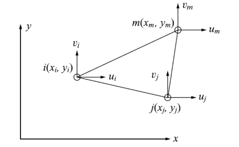
Select Displacement Functions

\[ u(x, y) = a_1 + a_2 x + a_3 y, \quad v(x, y) = a_4 + a_5 x + a_6 y \]

where \(a_i\) are constants. The strains are also constants:

\[ \varepsilon_x = a_2, \quad \varepsilon_y = a_6, \quad \gamma_{xy} = a_3 + a_5 \]

Hence the name "constant strain triangle".

Displacements at the 3 nodes:

\[ \begin{aligned} u_i &= u(x_i, y_i) = a_1 + a_2 x_i + a_3 y_i && v_i = v(x_i, y_i) = a_4 + a_5 x_i + a_6 y_i \\ u_j &= u(x_j, y_j) = a_1 + a_2 x_j + a_3 y_j && v_j = v(x_j, y_j) = a_4 + a_5 x_j + a_6 y_j \\ u_m &= u(x_m, y_m) = a_1 + a_2 x_m + a_3 y_m && v_m = v(x_m, y_m) = a_4 + a_5 x_m + a_6 y_m \end{aligned} \]

---

Create 2D Meshes in ABAQUS

• Part
  • Base Feature: Shell（面）
• Property
  • Create Section
  • Plane stress/strain thickness：只看最大应力的话，可以不设置；如果要求支座反力（需要用到厚度的），则需要设置。
• Assembly
  • Create Instance
    • Independent
• Step
  • Static, General
  • Nlgeoms：非线性，大变形
• Interaction
  • 多个 Part 之间的相互作用
• Load
  • Pressure（面载荷）
• Mesh

  • Element Type

    Reduced Integration（简缩积分）

    \(\mathbf{B}\) 一般是 \(x, y\) 的函数，会使用高斯数值积分方法。这个选项默认打开，会在单元内部使用较少的高斯积分点来减少计算量，同时尽可能保持良好的数值稳定性。但是简缩积分也可能引入数值问题，比如对 quad 元素会出现筛子效应。